Reflexxes Motion Libraries: The Position-based Type II On-Line Trajectory Generation Algorithm

This page contains four sections

A Brief Introduction

Input and output values of the Reflexxes Type II Motion Library in a generic manner.

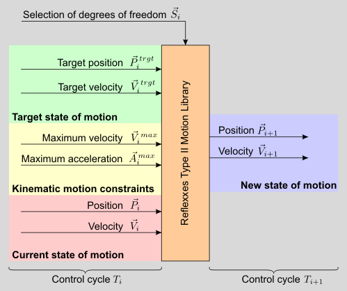
The interface (ReflexxesAPI) of all Reflexxes Motion Libraries is very simple and can easily be integrated into existing systems. Based on the current state of motion and the kinematic motion constraints, a new state of motion is calculated with lies exactly on the time-optimal trajectory to reach the desired target state of motion. All input values can change arbitrarily based on sensor signals and even discontinuously, and a steady jerk-limited motion trajectory is always guaranteed at the output The above figure shows the input and output values of the RML algorithm in a generic manner. It is the task of the algorithm to time-optimally transfer an arbitrary current state of motion

${\bf M}_{i}\,=\,\left(\vec{P}_{i},\, \vec{V}_{i},\, \vec{A}_{i} \right)$

into the desired target state of motion

${\bf M}_{i}^{\,trgt}\,=\,\left(\vec{P}_{i}^{\,trgt},\, \vec{V}_{i}^{\,trgt},\, \vec{0} \right)$

under consideration of the kinematic motion constraints

${\bf B}_{i}\,=\,\left( \vec{V}_{i}^{\,max},\, \vec{A}_{i}^{\,max},\, \vec{J}_{i}^{\,max} \right)$

The algorithm works memoryless and calculates only the next state of motion ${\bf M}_{i+1}$ , which is used as input value for lower-level motion controllers. The resulting trajectories are time-optimal and synchronized, such that all selected DOFs coinstantaneously reach their target state of motion. The selection vector $\vec{S}_i$ contains boolean values to mask single DOFs, for which no output values are calculated. All types and variant of the algorithm consist of three steps, which are introduced in the following.

For a better understanding of the basic algorithm for Type II On-Line Trajectory generation (OTG), this section presents a brief overview. For a detailed description, please refer to

T. Kroeger.
On-Line Trajectory Generation in Robotic Systems.
Springer Tracts in Advanced Robotics, Vol. 58, Springer, January 2010.
http://www.springer.com/978-3-642-05174-6

Step 1: Calculate the Synchronization Time

Although only one single scalar value is calculate in this step, it the the most complex one. First, the minimum execution times $_kt_{i}^{\,min}$ are calculated for each selected DOF $k \ \in\ \{1,\dots,K\}$ . The value of the minimum synchronization time $t_i^{\,sync}$ must be equal or greater than the minimum value of all minimum execution times. To transfer the motion state of one DOF to another, a finite set of motion profiles ${\cal P}_{Step1}$ is considered, and a decision tree selects a motion profile $_k\Psi_i^{\,Step1}\ \in\ {\cal P}_{Step1}$ for each selected DOF $k \ \in\ \{1,\dots,K\}$ . To calculate $_kt_{i}^{\,min}$ , a system of nonlinear equation is set-up, and the solution contains the desired value.

Depending on the type of the algorithm (I-IX), it may happen that up to $Z\,=\,3$ time intervals are existent, within which the target state of motion cannot be reached. For the Type II algorithm only $Z\,=\,1$ inoperative interval may be existent. The decision trees 1B and 1C are used to calculate all limits of these intervals $_k{\cal Z}_{i}$ , whose elements are denoted by

$_k^z\zeta_{i}\,=\,\left[^z_kt_{i}^{\,begin},\,^z_kt_{i}^{\,end}\right],\ \mbox{with}\ z\ \in\ \left\{1,\,\dots,\,Z\right\}$

Finally, the minimum time not being within any inoperative time interval

$_k^z\zeta_{i}\ \forall\ (z,\,k)\ \in \ \left\{1,\,\dots,\,Z\right\}\times\left\{1,\,\dots,\,K\right\}$

is selected as the value for the synchronization time $t_i^{\,sync}$ .

Step 2: Synchronization of All Selected DOFs

All selected DOFs that did not determine $t_i^{\,sync}$ have to be synchronized to this time value. In principal, an infinite number of solutions can be found to parameterize a trajectory that transfers such a DOF from $_k\vec{M}_i$ to $_k\vec{M}_i^{\,trgt}$ in $t_i^{\,sync}$ . In order to achieve a deterministic framework, an optimization criterion must be used in order to compute a time- or a phase-synchronized motion trajectory. Therefore, another decision tree is used, which selects a motion profile $_k\Psi_i^{\,Step2}$ for each DOF $ k $ from a different set that is denoted by ${\cal P}_{Step2}$ . Based on this profile, a nonlinear system of equations can be solved, and the solution contains all required parameters for the synchronized motion trajectory.

Step 3: Calculate Output Values

This last step is trivial: the resulting trajectory parameters of Step 2 are used to calculate a new state of motion ${\bf M}_{i+1}$ , which is used as set-point for lower-level controllers at $T_{i+1}$ .

Nassi-Shneiderman structogram of the basic OTG algorithm.

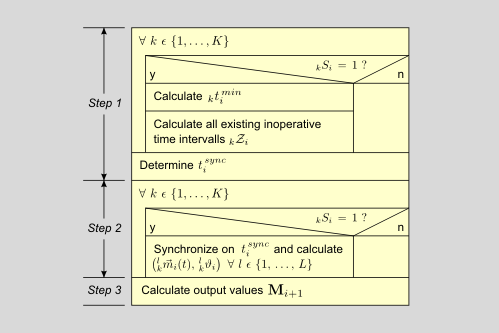
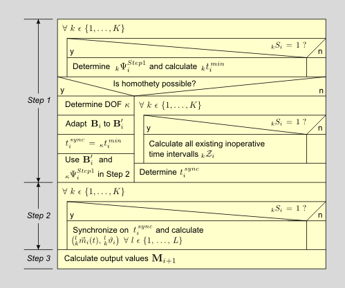
The figure above summarizes the generic version of the OTG algorithm for time-synchronization, while the figure below summarizes the version, in which phase-synchronization is applied.

Generic Nassi-Shneiderman structogram for the OTG algorithm for phase-synchronized trajectories.

The class ReflexxesAPI constitutes the actual user interface and provides the complete set of functionalities while hiding all parts of the library that are not required by the user. Users, who like to take a deeper look to the implementation of the algorithm, may learn about the class TypeIIRMLPosition and the namespace TypeIIRMLMath, both of which contain all mathematical details.